Podcast Trend Analysis -- Part 1
tl;dr:
I can start doing real analysis of trends in semantic-space, but slowly. It turns out that the queries I’m interested in are not necessarily suited to ANN-based approximations.
What?
By now, I’ve started to amass a decently large index of podcast content, enough to compute interesting statistics. Here are several examples of trends that my system is sensitive to.
The current implementation is naive: for a given query, the database scans every chunk of content and computes a relevance score for each, then these go into the statistics. This is slow, but it’s easy to reason about and performs predictably. A significantly faster way to do something similar would make use of the HNSW index to get the top-k approximate nearest neighbors to the query vector, then compute statistics exclusively from those k most relevant chunks, ignoring the “irrelevant” chunks entirely.
Indeed, that had been my plan from the beginning. With the exact queries working as expected, I could create their approximate equivalents and compare them to the exact variants empirically. However, I’ve been thinking about the degree and nature of information-loss that occurs as an inevitability of that approximation, and I’m starting to think the exact scanning approach may be more suitable.
The Case for Exactness
Using the HNSW index to run an approximate search for the top-k would almost certainly return a perfectly adequate top-k compared to the ground truth of running an exact scan and sorting by distance.1 For reasonable values of k, it will also be much faster.
What exactly is “a reasonable value of k”, though? In terms of speed (latency and throughput), a rule of thumb I see repeated is that when k < ~1% of N HNSW should reliably outperform an exact scan, and that by k > ~10% of N an exact scan starts to look preferable. Intuitively, this makes perfect sense to me simply by virtue of the sequential access pattern for an exact scan. Even in memory, random access (graph traversal, in this case) might easily reduce throughput by a factor of 10.2
This consideration of latency/throughput poses a question: essentially “what percentage of my data am I willing to ignore?”. If I can ignore ~99% of my data, k can be ~1% of N, and HNSW is a great deal. If I ignore merely ~90% of my data, k would be ~10% of N, and HNSW is no faster than an exact scan. Meanwhile, the exact scan can capture signal from 100% of my data.
In the case of a search for specific information, it’s very reasonable to ignore 99% of the data. In a trend analysis context, it’s often less reasonable. That’s not to say it’s anywhere near un-reasonable! In many real-world cases, the majority of the signal is in 1% of the data, and in some of those cases it’ll be the overwhelming majority of the signal. However, not all signals are so concentrated. This relates to the “broadness” or the “narrowness” of the topic, and how you want to treat relevance.
A “narrow” query is similar to tallying all the high-relevance search results of a specific area of concern, such as “new world-record for largest cabbage”. Chunks of content about cabbages generally, or even about unusually large cabbages, are irrelevant; we only want to find out when a new record has been set.
A “broad” query is something more like “deep-sea mining”, where we might even want to give some degree of fractional relevance to results about deep-sea minerals (even if mining isn’t mentioned) or to results about mining generally (even if it’s not strictly about the deep-sea). As long as we’re able to give correspondingly increased weight to results with correspondingly more relevance, there’s potential utility in such a signal.
For a closer look at how I’m handling fractional relevance, check out this section. There’s also a tangent about how HNSW interacts with filters, such as WHERE clauses in SQL, which was relevant in my decision to lean into exact scan processing.
In short, I think these “broad” queries are interesting, and I would like to be able to squeeze as much information out of them as possible. Doing this puts me into the realm where HNSW doesn’t have much advantage over an exact scan, and it results in non-zero information loss. At that point, an exact flat scan starts to look pretty good.
What’s next?
Making flat scans faster! Step one is more memory, step two is moving to something columnar (probably DuckDB). Eventually, I may want to run some experiments to handle NUMA better.
Appendix: Trend Examples
The RAMpocalypse 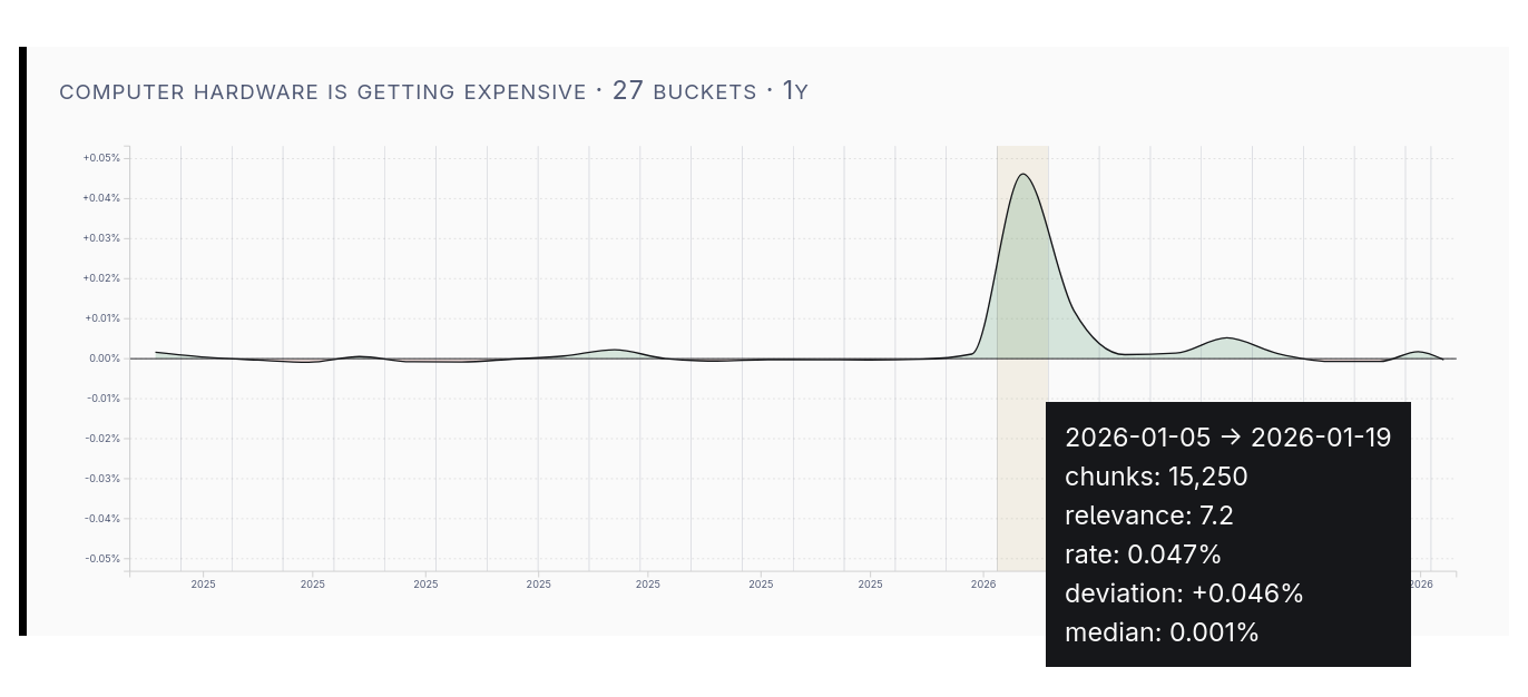
This spike in podcast coverage of “computer hardware getting expensive” lines up with the surge in memory prices.
Which feeds are “scary true crime”? 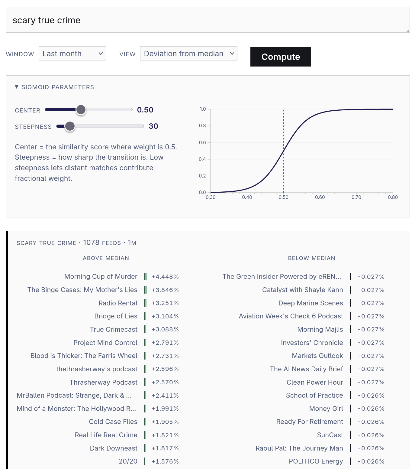
This view compares the relevance-rate of chunks on a by-feed basis. The left column shows the feeds that are most above the median rate, and the right column shows the feeds that are the most below the median rate. If you’re curious about those “sigmoid parameters”, check out the explanation.
AI Models from China? 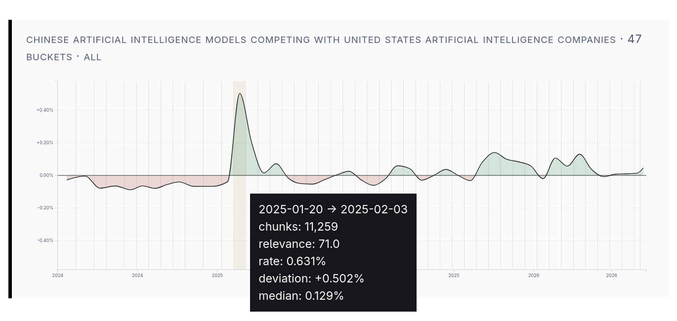
Do you remember when everyone was talking about DeepSeek? I myself didn’t remember precisely when, but the data clearly indicates it was January 2025.
Tariffs 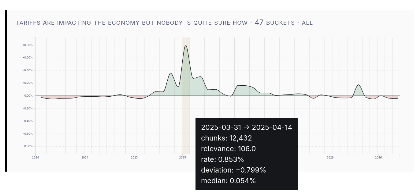
This chart shows something that I recall: podcasts talked about tariffs for a longer period of time than they talked about DeepSeek. Of course the main spike occurs around April 2, but we can see a lasting elevation.
Financial News Coverage 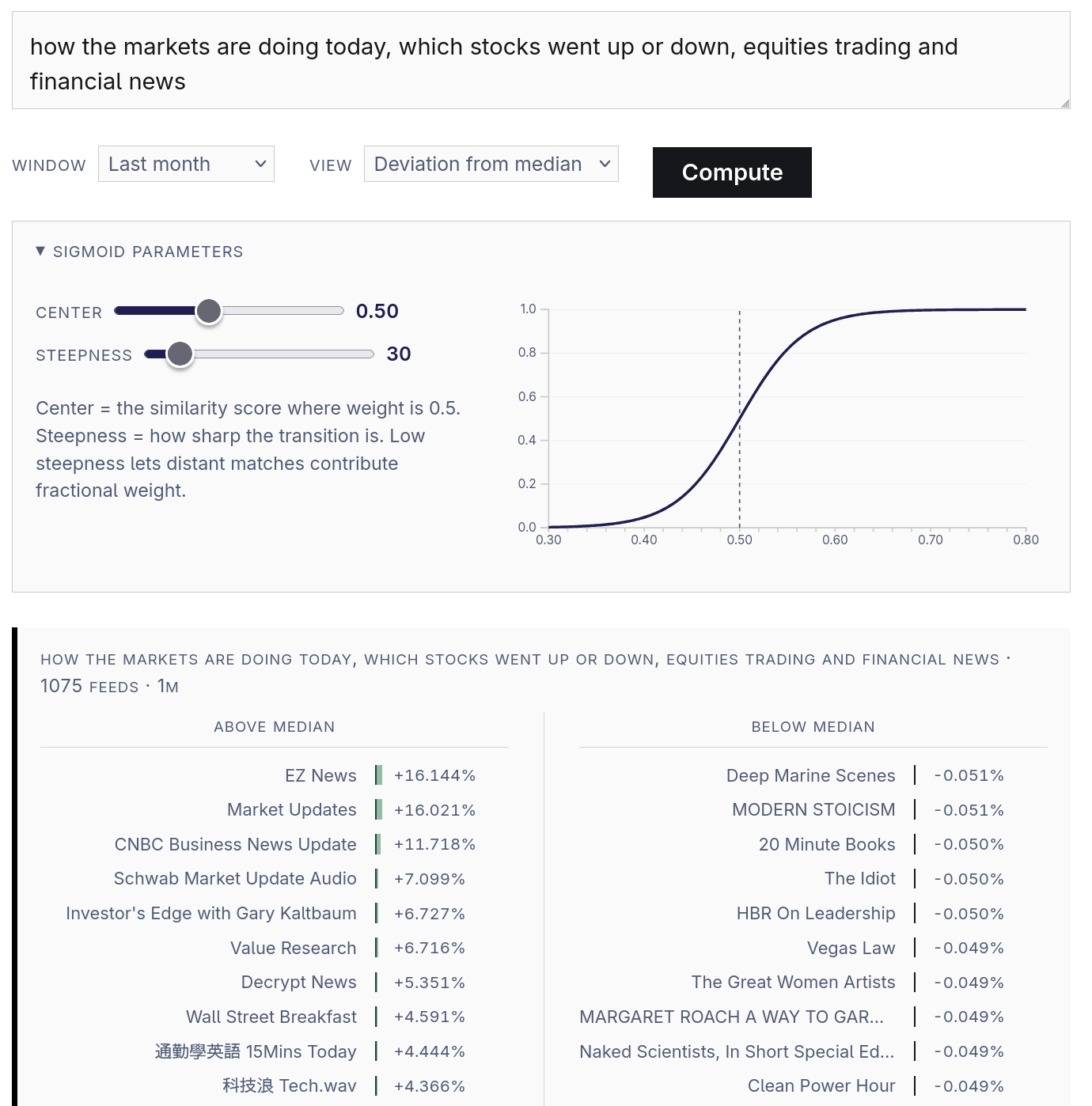
This EZ News show seems to open every episode with a stock quote. Predictably, the Stoics don’t talk much about stocks.
Build Notes
Trends Queries
You can check out the source, but there’s not too much to know performance-wise: queries are flat, exact scans. The table is currently around 16GB. When it’s sitting on the disk and not cached (such as on a cheap VPS without that much RAM), the absolute upper bound for performance is simply how fast you can read 16GB off the disk. Even if this was a perfectly sequential access pattern (which it isn’t), on a fast disk, the query would take multiple seconds.
Without thinking deeply about Postgres internals, I know that, at a minimum, the vectors I need are TOAST‘d, so there’s at least one layer of indirection between them and being sequentially flat scanned. In reality, I can be certain just by the readily observable runtime performance characteristics and background knowledge that there’s more indirection than that!
There’s more than one way I could make the scan faster in Postgres. The only one I had been seriously considering was to use ANN to approximate my query. Having decided against that for now, I think it’s time to admit that I am clearly in OLAP territory, and I should probably stop trying to get good results from an OLTP-leaning database.
Filtering
With a single HNSW index on a single table, you don’t necessarily gain performance from filtering out a lot of rows. In fact, with pgvector (and presumably other implementations), you lose performance! Essentially, the ANN step of the query has to be first, because the HNSW graph is not aware of anything but the vectors themselves. Filters are applied afterward, to the k results returned.
For a concrete example, I have a table with content-chunks stretching back over 18 months. If I want to compute statistics over the last 1 month, I don’t get to chop the table down to 1/18th of its size and then run ANN on that small piece.
If you want the 1,000 approximate-nearest results from the entire date range, you can simply query with k=1,000 and get the result that you want. If instead you want the 1,000 approximate-nearest results within 1 given month out of the 18 you’d need to use much larger k. In this scenario, you could try k=18,000 on the assumption that the results are evenly distributed across time. However, even a cursory glance will show this to be a visibly poor assumption.3 So, even with a filter which isn’t very selective, you might find k growing out of control very quickly, depending on how the data is distributed.
This of course interacts very poorly with everything I wrote about earlier.
Pgvector does have iterative index scans, but that’s not the same thing as filter-aware traversal. If I understand correctly, it’s just to keep you from having to guess the right k ahead of time: dynamically extending the traversal until enough candidates survive filtering. It looks like Qdrant and Weaviate are doing something more like “filter-aware traversal”.
At a glance, it looks like they are likely outperforming pgvector in the sense that you can apply filters that are more selective before you fall into the territory where a scan beats ANN. My impression is that they’re buying more ground for the general case of filtering, but, if I wanted to run the fastest approximate queries in the very specific case I described above, I might be better served by simply giving each month of data its own HNSW index.
Spatial Decay
Before I had thought about it much, I figured it would be interesting to show trends in terms of how many relevant results existed in a given feed, or in a given time period to create something like the charts above. I quickly had to confront the question: what is “relevant”, exactly?
One might use a threshold. With the embedding model that I’m using, the vibes are roughly so:
| Similarity Score | Search Result Quality |
|---|---|
| 0.45 or lower | not likely good |
| 0.5 | might be good |
| 0.55 | likely good |
| 0.6 or higher | very likely good |
Why not use 0.55 as a threshold and count the results? This is not unreasonable, but it is discarding information that might be useful. It’s collecting only 1 bit of information per chunk of content. For your consideration, here’s what a photographic image looks like when each pixel carries only one bit of information:
Aside from a straightforward loss of information, the result is sensitive to where you set the threshold. If you set it wrong, you can completely miss what you’re looking for.
If you want to see how far even just a little information can go, try “4-bit” mode where there are 16 distinct values that a pixel can have. The image should be quite clear to your eye.
Finally, try switching to the sigmoid mode. If you set “steepness” very low, you should be able to see the flower pretty clearly no matter how you move “center”. However, with the steepness set to a low number, you can see there’s not much contrast in the image.
Start to crank up the steepness, and you’ll get contrast – but now it’s much more important where “center” is set.
Trying to view a trend in this podcast data is a little bit like trying to determine which regions of that image are the flower versus the background. It’s hard to trace the outline of the flower with 1-bit per pixel. It’s a bit easier with more information. It’s even easier if you set center=95 and steepness=50, amplifying the differences that separate the subject from the background. That’s essentially what the sigmoid function is doing when applied to the similarity scores of each chunk of podcast content.
There's no formal bound for the loss of recall performance with HNSW compared to an exact scan, but there's a generally established view that it works well in practice, and, of course, you can measure an epsilon with respect to your data.
Thinking about it a bit more deeply, `ef_search` (an HNSW parameter applied per query) needs to increase as `k` increases to maintain similar result quality. This definitely costs latency, at least linearly in proportion to the value. I'm fairly certain there'll also be a sharp nonlinearity somewhere: above some value of `ef_search`, important bits of query state will start falling out of the CPU cache.
Of course, there may be some datasets and some types of filters where this assumption holds.